Introductory Notes
Before diving into how you can access the 3D dust map, we'd like to make you aware of a few important points about the dataset.
Versions
There are three versions of the 3D dust map, which we refer to as Bayestar19 (Green et al. 2019), Bayestar17 (Green et al. 2018) and Bayestar15 (Green et al. 2015). Please refer to the papers for detailed differences between the maps.
Units
The units of Bayestar19, Bayestar17 and Bayestar15 differ. This is primarily due to the different extinction laws assumed by the three versions of the dust map. While Bayestar19 and Bayestar17 assume the slightly different versions of the reddening vector derived by Schlafly et al. (2016), Bayestar15 relies on the extinction relations of Fitzpatrick (1999) and Cardelli et al. (1989). All three versions of the map are intended to provide reddening in a similar unit as SFD (Schlegel et al. 1998), which is not quite equal to E(B-V ) (see the recalibration of SFD undertaken in Schlafly & Finkbeiner 2011).
Bayestar19
In order to convert Bayestar19 to extinction in Pan-STARRS 1 or 2MASS passbands, multiply the value reported by the map by the following coefficients:
| g | r | i | z | y | J | H | Ks |
|---|---|---|---|---|---|---|---|
| 3.518 | 2.617 | 1.971 | 1.549 | 1.263 | 0.7927 | 0.4690 | 0.3026 |
In order to convert to extinction or reddening in other passbands, one must assume some relation between extinction in Pan-STARRS 1 or 2MASS passbands and other passbands. For example, applying the RV = 3.1 Fitzpatrick (1999) reddening law to a 7000 K source spectrum, as done in Table 6 of Schlafly & Finkbeiner (2011), one obtains the relations
| E(B-V ) = 0.981 E(g-r )P1, | (1) |
| E(B-V ) = 0.932 E(r-z )P1. | (2) |
Because the Fitzpatrick (1999) reddening law is different from the reddening law we assumed when producing Bayestar19, the two above relations give slightly different conversions between the values reported by Bayestar19 and E(B-V ). Using Eq. (1), we find that E(B-V ) = 0.884 × (Bayestar19). Using Eq. (2), we find that E(B-V ) = 0.996 × (Bayestar19).
The overall normalization of Bayestar19 was chosen so that one unit of Bayestar19 reddening predicts the same E(g-r ) as one unit of the original SFD reddening map. That means that if one assumes Eq. (1) to hold, then Bayestar19 is equivalent to SFD, and reddening in non-PS1 passbands can be obtained by multiplying Bayestar19 by the coefficients in Table 6 of Schlafly & Finkbeiner (2011).
Bayestar17
In order to convert Bayestar17 to extinction in Pan-STARRS 1 or 2MASS passbands, multiply the value reported by the map by the following coefficients:
| g | r | i | z | y | J | H | Ks |
|---|---|---|---|---|---|---|---|
| 3.384 | 2.483 | 1.838 | 1.414 | 1.126 | 0.650 | 0.327 | 0.161 |
Just as with Bayestar19, the normalization of Bayestar17 was chosen to predict the same E(g-r ) as one unit of the original SFD reddening map, so Eqs. (1) and (2) above also hold for Bayestar17, and reddening in non-PS1 passbands can be obtained by multiplying Bayestar17 by the coefficients in Table 6 of Schlafly & Finkbeiner (2011).
Bayestar15
In contrast, Bayestar15 reports uses the same units as Schlegel, Finkbeiner & Davis (1998) reddenings. Although this was originally supposed to be the excess B-V in the Landolt filter system, Schlafly & Finkbeiner (2011) found that it differs somewhat from the true stellar B-V excess. Therefore, in order to convert our values of E(B-V ) to extinction in various filter systems, consult Table 6 of Schlafly & Finkbeiner (2011) (use the values in the RV = 3.1 column), which are based on the Fitzpatrick (1999) reddening law. For 2MASS passbands, Bayestar15 assumes a Cardelli et al. (1989) reddening law.
The extinction coefficients assumed by Bayestar15 are as follows:
| g | r | i | z | y | J | H | Ks |
|---|---|---|---|---|---|---|---|
| 3.172 | 2.271 | 1.682 | 1.322 | 1.087 | 0.786 | 0.508 | 0.320 |
Gray component of extinction vector
Note that the Bayestar15 extinction coefficients differ more from those used by Bayestar17 in the near-infrared than in the optical. This is due to the uncertainty in the gray component of the extinction vector (corresponding to an overall additive change to all extinction coefficients), which is not as well constrained as the ratios of reddenings in different filter combinations. For example, the ratio of E(g-r ) to E(J-K ) is better constrained than Ag, Ar, AJ or AKs individually. Because the near-infrared extinction coefficients are smaller than those at optical wavelengths, near-infrared extinction estimates are more affected (percentually) by uncertainty in the gray component than optical extinctions.
The Bayestar17 extinction coefficients were derived under the assumption of zero reddening in the WISE W2 passband. This necessarily produces an underestimate of the gray component of the extinction vector. If one instead assumes that AH / AK = 1.55 (Indebetouw et al. 2005), then an additional 0.141 should be added to all of the Bayestar17 extinction coefficients. If one assumes that AH / AK = 1.74 (Nishiyama et al. 2006), then one should add in 0.063 to all of the Bayestar17 extinction coefficients. The gray component that should be added into the Bayestar17 extinction coefficients is therefore in the range 0 ≲ ΔR ≲ 0.141.
The differences between the extinction vectors assumed by Bayestar19 and Bayestar17 are due in part to their use of slightly different reddening vectors, but are dominated by their different choice in normalization of the gray component of the extinction vector. While Bayestar19 assumes that AH / AK = 1.55 (Indebetouw et al. 2005), Bayestar17 assumes that there is zero extinction in the WISE W2 passband.
Samples
For each sightline, we provide multiple estimates of the distance vs. reddening relationship. Alongside the maximum-probability density estimate (essentially, the best-fit) distance-reddening curve, we also provide samples of the distance-reddening curve, which are representative of the formal uncertainty in the relation. Most statistics you may wish to derive, like the median reddening to a given distance, are best determined by using the representative samples, rather than the best-fit relation.
Quality Assurance
We include a number of pieces of information on the reliability of each pixel. A convergence flag marks whether our fit to the line-of-sight reddening curve converged. This is a formal indicator, meaning that we correctly sampled the spread of possible distance-reddening relations, given our model assumptions. It does not, however, indicate that our model assumptions were correct for that pixel. This convergence flag is based on the Gelman-Rubin diagnostic, a method of flagging Markov Chain Monte Carlo non-convergence.
Additionally, minimum and maximum reliable distances are provided for each pixel, based on the distribution of stars along the sightline. Because we determine the presence of dust by observing differential reddening of foreground and background stars, we cannot trace dust beyond the farthest stars in a given pixel. Our estimates of dust reddening closer than the nearest observed stars in a pixel are similarly uncertain. We therefore urge caution in using our maps outside of the distance range indicated for each pixel.
Accessing the Map
The Python package dustmaps provides functions both for querying Bayestar15/17/19 and for downloading the maps. The dustmaps package also makes a number of additional 3D and 2D dust maps available through a uniform framework. For users who do not wish to download the entire Bayestar15/17/19 maps, dustmaps provides functions for querying these maps remotely.
After installing dustmaps and fetching the Bayestar data cubes, one can query it as follows:
>>> from astropy.coordinates import SkyCoord
>>> import astropy.units as units
>>> from dustmaps.bayestar import BayestarQuery
>>>
>>> bayestar = BayestarQuery(version='bayestar2017') # 'bayestar2019' is the default
>>> coords = SkyCoord(90.*units.deg, 30.*units.deg,
...                   distance=100.*units.pc, frame='galactic')
>>>
>>> reddening = bayestar(coords, mode='median')
>>> print(reddening)
0.00621500005946
If you prefer not to download the full Bayestar data cubes, you can query the map remotely:
>>> from astropy.coordinates import SkyCoord
>>> import astropy.units as units
>>> from dustmaps.bayestar import BayestarWebQuery
>>>
>>> bayestar = BayestarWebQuery(version='bayestar2017')
>>> coords = SkyCoord(90.*units.deg, 30.*units.deg,
...                   distance=100.*units.pc, frame='galactic')
>>>
>>> reddening = bayestar(coords, mode='random_sample')
>>> print(reddening)
0.00590000022203
The above code will contact our server to retrieve only the coordinates you're interested in. If you're interested in only a few - or even a few thousand - coordinates, this is the most efficient way to query the map.
Using dustmaps, you can also query multiple coordinates at once. For example, the following snippet of code remotely queries the 90ᵗʰ percentile of reddening in the Bayestar17 map at an array of coordinates:
>>> import numpy as np
>>> from astropy.coordinates import SkyCoord
>>> import astropy.units as units
>>> from dustmaps.bayestar import BayestarWebQuery
>>>
>>> bayestar = BayestarWebQuery() # Uses Bayestar2017 by default.
>>>
>>> l = np.array([30., 60., 90.])
>>> b = np.array([-15., 10., 70.])
>>> d = np.array([0.1, 3., 0.5])
>>> coords = SkyCoord(l*units.deg, b*units.deg,
...                   distance=d*units.kpc, frame='galactic')
>>>
>>> reddening = bayestar(coords, mode='percentile', pct=90.)
>>> print(reddening)
[ 0.085303    0.22474321  0.03297591]
The dustmaps package can be used to query a number of dust maps beyond Bayestar15/17/19. For example, you can query Schlegel, Finkbeiner & Davis (1998), either from a version stored on local disk or remotely:
>>> from astropy.coordinates import SkyCoord
>>> import astropy.units as units
>>> from dustmaps.sfd import SFDWebQuery
>>>
>>> sfd = SFDWebQuery()
>>> coords = SkyCoord(45.*units.deg, 45.*units.deg, frame='icrs') # Equatorial
>>>
>>> ebv_sfd = sfd(coords)
>>> print(ebv_sfd)
0.22122733295
See the dustmaps documentation for more information.
Legacy Query Code
If you prefer not to download the dustmaps Python package, or if you don't use Python, you can still remotely query the older version of our map, Bayestar15, with the following function, given in both Python and IDL. We strongly recommend the dustmaps package, but the following code is an alternative way to access the older Bayestar15 map.
Function Call
import json, requests

def query(lon, lat, coordsys='gal', mode='full'):
    '''
    Send a line-of-sight reddening query to the Argonaut web server.

    Inputs:
      lon, lat: longitude and latitude, in degrees.
      coordsys: 'gal' for Galactic, 'equ' for Equatorial (J2000).
      mode: 'full', 'lite' or 'sfd'

    In 'full' mode, outputs a dictionary containing, among other things:
      'distmod':    The distance moduli that define the distance bins.
      'best':       The best-fit (maximum proability density)
                    line-of-sight reddening, in units of SFD-equivalent
                    E(B-V), to each distance modulus in 'distmod.' See
                    Schlafly & Finkbeiner (2011) for a definition of the
                    reddening vector (use R_V = 3.1).
      'samples':    Samples of the line-of-sight reddening, drawn from
                    the probability density on reddening profiles.
      'success':    1 if the query succeeded, and 0 otherwise.
      'converged':  1 if the line-of-sight reddening fit converged, and
                    0 otherwise.
      'n_stars':    # of stars used to fit the line-of-sight reddening.
      'DM_reliable_min':  Minimum reliable distance modulus in pixel.
      'DM_reliable_max':  Maximum reliable distance modulus in pixel.

    Less information is returned in 'lite' mode, while in 'sfd' mode,
    the Schlegel, Finkbeiner & Davis (1998) E(B-V) is returned.
    '''

    url = 'http://argonaut.skymaps.info/gal-lb-query-light'

    payload = {'mode': mode}

    if coordsys.lower() in ['gal', 'g']:
        payload['l'] = lon
        payload['b'] = lat
    elif coordsys.lower() in ['equ', 'e']:
        payload['ra'] = lon
        payload['dec'] = lat
    else:
        raise ValueError("coordsys '{0}' not understood.".format(coordsys))

    headers = {'content-type': 'application/json'}

    r = requests.post(url, data=json.dumps(payload), headers=headers)

    try:
        r.raise_for_status()
    except requests.exceptions.HTTPError as e:
        print('Response received from Argonaut:')
        print(r.text)
        raise e

    return json.loads(r.text)
This code can be adapted for any programming language that can issue HTTP POST requests. The code can also be found on GitHub.
Example Usage
To query one sightline, say, Galactic coordinates (ℓ, b) = (90°, 10°), you would call
>>> # Query the Galactic coordinates (l, b) = (90, 10):
>>> qresult = query(90, 10, coordsys='gal')
>>>
>>> # See what information is returned for each pixel:
>>> qresult.keys()
[u'b', u'GR', u'distmod', u'l', u'DM_reliable_max', u'ra', u'samples',
u'n_stars', u'converged', u'success', u'dec', u'DM_reliable_min', u'best']
>>>
>>> qresult['n_stars']
750
>>> qresult['converged']
1
>>> # Get the best-fit E(B-V) in each distance slice
>>> qresult['best']
[0.00426, 0.00678, 0.0074, 0.00948, 0.01202, 0.01623, 0.01815, 0.0245,
0.0887, 0.09576, 0.10139, 0.12954, 0.1328, 0.21297, 0.23867, 0.24461,
0.37452, 0.37671, 0.37684, 0.37693, 0.37695, 0.37695, 0.37696, 0.37698,
0.37698, 0.37699, 0.37699, 0.377, 0.37705, 0.37708, 0.37711]
>>>
>>> # See the distance modulus of each distance slice
>>> qresult['distmod']
[4.0, 4.5, 5.0, 5.5, 6.0, 6.5, 7.0, 7.5, 8.0, 8.5, 9.0, 9.5, 10.0, 10.5,
11.0, 11.5, 12.0, 12.5, 13.0, 13.5, 14.0, 14.5, 15.0, 15.5, 16.0, 16.5,
17.0, 17.5, 18.0, 18.5, 19.0]
You can also query multiple sightlines simultaneously, simply by passing longitude and latitude as lists:
>>> qresult = query([45, 170, 250], [0, -20, 40])
>>>
>>> qresult['n_stars']
[352, 162, 254]
>>> qresult['converged']
[1, 1, 1]
>>> # Look at the best fit for the first pixel:
>>> qresult['best'][0]
[0.00545, 0.00742, 0.00805, 0.01069, 0.02103, 0.02718, 0.02955, 0.03305,
0.36131, 0.37278, 0.38425, 0.41758, 1.53727, 1.55566, 1.65976, 1.67286,
1.78662, 1.79262, 1.88519, 1.94605, 1.95938, 2.0443, 2.39438, 2.43858,
2.49927, 2.54787, 2.58704, 2.58738, 2.58754, 2.58754, 2.58755]
If you are going to be querying large numbers of sightlines at once, we kindly request that you use this batch syntax, rather than calling query() in a loop. It will be faster, because you only have to contact the server once, and it will reduce the load on the Argonaut server.
Two additional query modes are provided, beyond the default 'full' mode. If mode = 'lite' is passed to the query() function, then less information is returned per sightline:
>>> qresult = query(180, 0, coordsys='gal', mode='lite')
>>> qresult.keys()
[u'b', u'success', u'distmod', u'sigma', u'median', u'l',
u'DM_reliable_max', u'ra', u'n_stars', u'converged', u'dec',
u'DM_reliable_min', u'best']
>>>
>>> # Get the median E(B-V) to each distance slice:
>>> qresult['median']
[0.0204, 0.02747, 0.03027, 0.03036, 0.03047, 0.05214, 0.05523, 0.0748,
0.07807, 0.10002, 0.13699, 0.2013, 0.20158, 0.20734, 0.23129, 0.73734,
0.76125, 0.83905, 0.90236, 1.05944, 1.08085, 1.11408, 1.11925, 1.12212,
1.12285, 1.12289, 1.12297, 1.12306, 1.12308, 1.12309, 1.12312]
>>>
>>> # Get the standard deviation of E(B-V) in each slice
>>> # (actually, half the difference between the 84th and 16th percentiles):
>>> qresult['sigma']
[0.03226, 0.03476, 0.03452, 0.03442, 0.03439, 0.03567, 0.03625, 0.0317,
0.03238, 0.03326, 0.05249, 0.0401, 0.03919, 0.03278, 0.08339, 0.05099,
0.03615, 0.04552, 0.05177, 0.03678, 0.03552, 0.05246, 0.05055, 0.05361,
0.05422, 0.0538, 0.05381, 0.05381, 0.0538, 0.0538, 0.05379]
Finally, for the convenience of many users who also want to query the two-dimensional Schlegel, Finkbeiner & Davis (1998) map of dust reddening, the option mode = 'sfd' is also provided:
>>> qresult = query([0, 10, 15], [75, 80, 85], coordsys='gal', mode='sfd')
>>>
>>> qresult.keys()
[u'EBV_SFD', u'b', u'dec', u'l', u'ra']
>>>
>>> # E(B-V), in magnitudes:
>>> qresult['EBV_SFD']
[0.02119, 0.01813, 0.01352]
Download Data Cube
If you prefer to work with the entire 3D map directly, rather than using the Python package dustmaps, you can obtain the data cube in either HDF5 or FITS format from the Harvard Dataverse: Bayestar19, Bayestar17 and Bayestar15.
Each map comes to several Gigabytes in compressed HDF5 format, so if you're only interested in individual (or even a few thousand) sightlines, we strongly recommend you use the remote query API in the dustmaps package.
Reading HDF5 Data Cube
The HDF5 format is a self-documenting, highly flexible format for scientific data. It has a number of powerful features, such as internal compression and compound datatypes (similar to numpy structured arrays), and has bindings in many different programming languages, including C, Python, Fortran and IDL.
The HDF5 file we provide has four datasets:
- /pixel_info : pixel locations and metadata.
- /samples : samples of distance vs. reddening profile in each pixel.
- /best_fit : best-fit distance vs. reddening profile in each pixel.
- /GRDiagnostic : Gelman-Rubin convergence diagnostic in each pixel (only in Bayestar15/17).
All four datasets are ordered in the same way, so that the nth element of the /samples dataset corresponds to the same pixel as described by the nth entry in /pixel_info. As our 3D dust map contains pixels of different sizes, /pixel_info specifies each pixel by a HEALPix nside and nested pixel index.
An example in Python will help illustrate the structure of the file:
>>> import numpy as np
>>> import h5py
>>>
>>> f = h5py.File('dust-map-3d.h5', 'r')
>>> pix_info = f['/pixel_info'][:]
>>> samples = f['/samples'][:]
>>> best_fit = f['/best_fit'][:]
>>> GR = f['/GRDiagnostic'][:]
>>> f.close()
>>>
>>> print(pix_info['nside'])
[512 512 512 ..., 1024 1024 1024]
>>>
>>> print(pix_info['healpix_index'])
[1461557 1461559 1461602 ..., 6062092 6062096 6062112]
>>>
>>> print(pix_info['n_stars'])
[628 622 688 ..., 322 370 272]
>>>
>>> # Best-fit E(B-V) in each pixel
>>> best_fit.shape  # (# of pixels, # of distance bins)
(2437292, 31)
>>>
>>> # Get the best-fit E(B-V) in each distance bin for the first pixel
>>> best_fit[0]
array([ 0.00401   ,  0.00554   ,  0.012     ,  0.01245   ,  0.01769   ,
        0.02089   ,  0.02355   ,  0.03183   ,  0.04297   ,  0.08127   ,
        0.11928   ,  0.1384    ,  0.95464998,  0.9813    ,  1.50296998,
        1.55045998,  1.81668997,  1.86567998,  1.9109    ,  2.00281   ,
        2.01739001,  2.02519011,  2.02575994,  2.03046989,  2.03072   ,
        2.03102994,  2.03109002,  2.03109002,  2.03110003,  2.03110003,
        2.03111005], dtype=float32)
>>>
>>> # Samples of E(B-V) from the Markov Chain
>>> samples.shape  # (# of pixels, # of samples, # of distance bins)
(2437292, 20, 31)
>>>
>>> # The Gelman-Rubin convergence diagnostic in the first pixel.
>>> # Each distance bin has a separate value.
>>> # Typically, GR > 1.1 indicates non-convergence.
>>> GR[0]
array([ 1.01499999,  1.01999998,  1.01900005,  1.01699996,  1.01999998,
        1.01999998,  1.02400005,  1.01600003,  1.00800002,  1.00600004,
        1.00100005,  1.00199997,  1.00300002,  1.02499998,  1.01699996,
        1.00300002,  1.01300001,  1.00300002,  1.00199997,  1.00199997,
        1.00199997,  1.00199997,  1.00100005,  1.00100005,  1.00100005,
        1.00100005,  1.00100005,  1.00100005,  1.00100005,  1.00100005,
        1.00100005], dtype=float32)
Example Usage
As a simple example of how to work with the full data cube, we will plot the median reddening in the farthest distance bin. We begin by opening the HDF5 file and extracting the information we need:
>>> import numpy as np
>>> import h5py
>>> import healpy as hp
>>> import matplotlib.pyplot as plt
>>>
>>> # Open the file and extract pixel information and median reddening in the far limit
>>> f = h5py.File('dust-map-3d.h5', 'r')
>>> pix_info = f['/pixel_info'][:]
>>> EBV_far_median = np.median(f['/samples'][:,:,-1], axis=1)
>>> f.close()
The variable pix_info specifies the location of each pixel (by nside and healpix_index), while EBV_far_median contains the median reddening in each pixel in the farthest distance bin. We want to construct a single-resolution HEALPix map, which we can use standard library routines to plot.
We find the maximum nside present in the map, and create an empty array, pix_val, to house the upsampled map:
>>> # Construct an empty map at the highest HEALPix resolution present in the map
>>> nside_max = np.max(pix_info['nside'])
>>> n_pix = hp.pixelfunc.nside2npix(nside_max)
>>> pix_val = np.empty(n_pix, dtype='f8')
>>> pix_val[:] = np.nan
Now, we have to fill the upsampled map, by putting every pixel in the original map into the correct location(s) in the upsampled map. Because our original map has multiple resolutions, pixels that are below the maximum resolution correspond to multiple pixels in the upsampled map. We loop through the nside resolutions present in the original map, placing all the pixels of the same resolution into the upsampled map at once:
>>> # Fill the upsampled map
>>> for nside in np.unique(pix_info['nside']):
...     # Get indices of all pixels at current nside level
...     idx = pix_info['nside'] == nside
...
...     # Extract E(B-V) of each selected pixel
...     pix_val_n = EBV_far_median[idx]
...
...     # Determine nested index of each selected pixel in upsampled map
...     mult_factor = (nside_max/nside)**2
...     pix_idx_n = pix_info['healpix_index'][idx] * mult_factor
...
...     # Write the selected pixels into the upsampled map
...     for offset in range(mult_factor):
...         pix_val[pix_idx_n+offset] = pix_val_n[:]
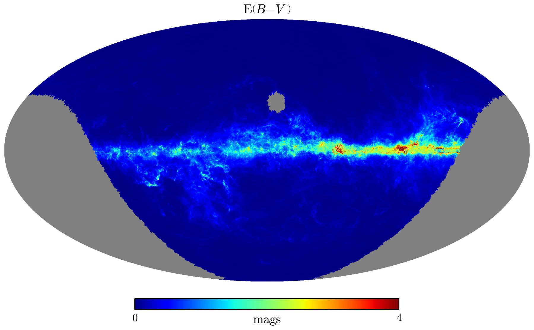
Now we have an array, pix_val, that represents reddening in the farthest distance bin. We can use one of healpy's built-in visualization functions to plot the map:
>>> # Plot the results using healpy's matplotlib routines
>>> hp.visufunc.mollview(pix_val, nest=True, xsize=4000,
                         min=0., max=4., rot=(130., 0.),
                         format=r'$%g$',
                         title=r'$\mathrm{E} ( B-V \, )$',
                         unit='$\mathrm{mags}$')
>>> plt.show()
Here's the resulting map. Note that it's centered on (ℓ, b) = (130°, 0°):
License
All code snippets included on this page are covered by the MIT License. In other words, feel free to use the code provided here in your own work.